Ground-motion modeling
Validating Ground-Motion Simulations
Testing how well Southern California’s 3D velocity models reproduce observed shaking, from regional patterns to basin amplification and surface-wave arrivals.
- Python
- Model Validation
- HPC
Research question
Where do widely used 3D velocity models reproduce observed ground motion, and which physical features explain their failures?
Study design
I designed and conducted a validation study of CVM-SI and CVM-H using 15,548 seismic records from 188 earthquakes and 1,719 stations. I built the Python, Bash, and Slurm workflows to run 3D spectral-element simulations and compare their output with observed ground motion.
Rather than collapsing model performance into one score, I examined amplitude, duration, arrival timing, and waveform shape separately, then investigated how the mismatches vary across Southern California’s basins.
Key findings
Model rankings depend on what is measured
Both models reproduce broad regional patterns, but their agreement with observations changes with location, frequency, and waveform property. Keeping the metrics separate reveals errors that an overall score obscures.
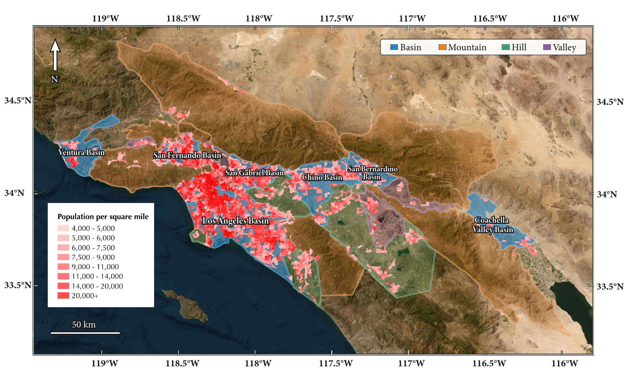
Basin amplification has distinct biases
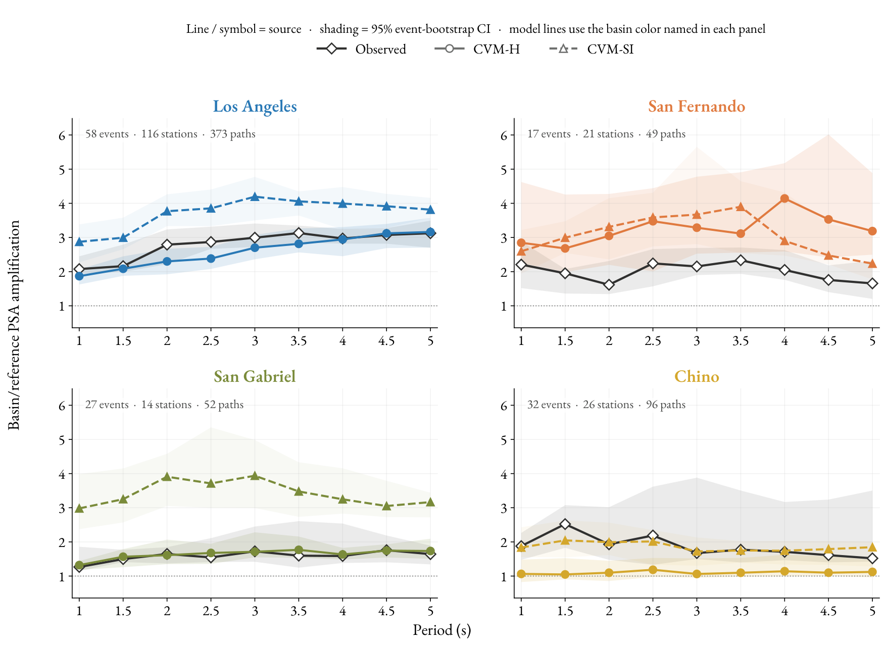
CVM-SI generally overamplifies peak and spectral accelerations in the Los Angeles and San Gabriel basins. CVM-H generally underamplifies peak acceleration and more closely matches the observed Los Angeles response-spectral amplification. The same biases do not hold in every basin.
Some observed surface waves are missing
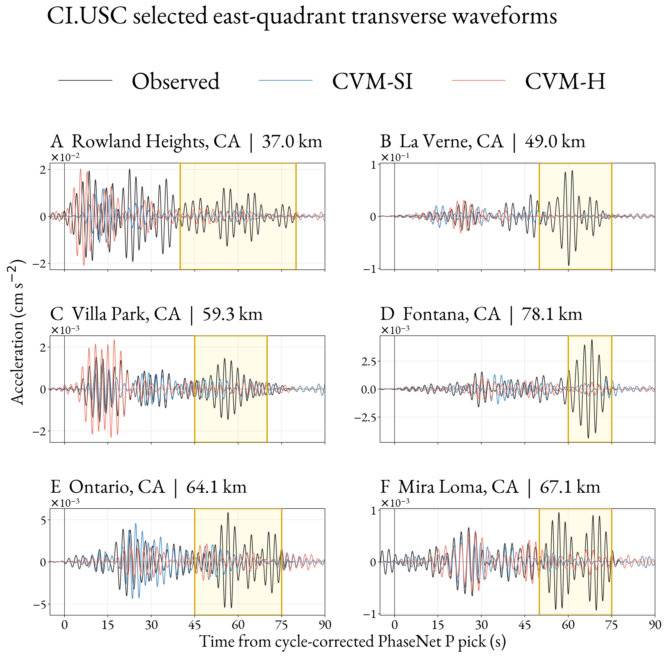
For several earthquakes east of Los Angeles, records at station CI.USC contain a coherent late transverse Love-wave packet that is weak or absent in both sets of simulations.
Two models represent basin structure differently
CVM-SI combines a comparatively smooth tomographic model with a shallow geotechnical layer. CVM-H embeds detailed basin structures derived from reflection data within a regional tomographic background. The rotating views show how differently the two meshes represent the same region.
Basin amplification exposes local model biases
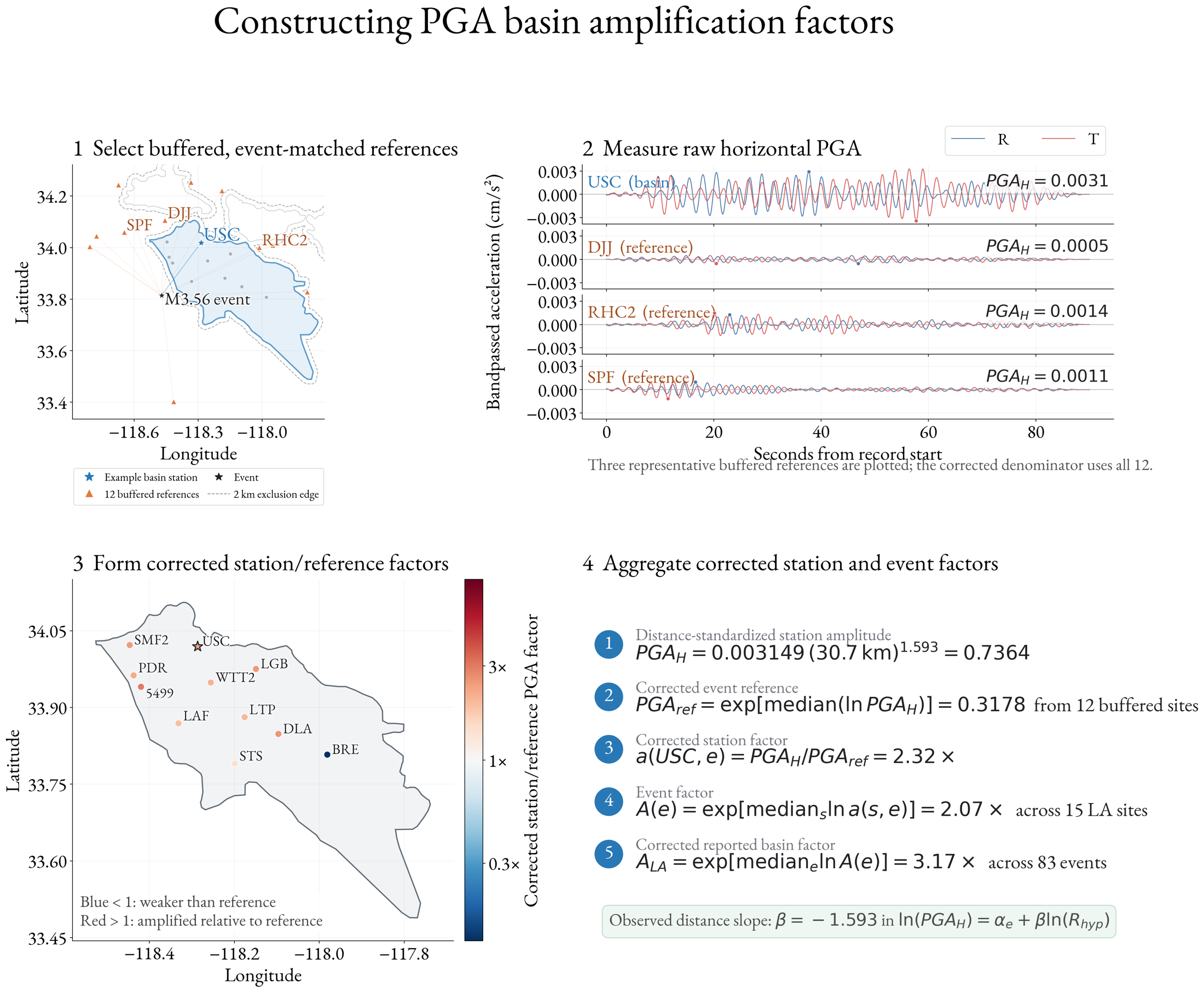
I compared basin stations with hard-rock reference stations outside each basin, corrected for distance differences, and combined measurements across events. This isolates basin-scale amplification more clearly than a map of raw amplitudes.
CVM-SI generally overamplifies shaking in the Los Angeles and San Gabriel basins. CVM-H’s performance varies by basin and period, showing why a model that works well in one basin cannot simply be assumed to work equally well in another.
Waveforms reveal missing surface-wave arrivals
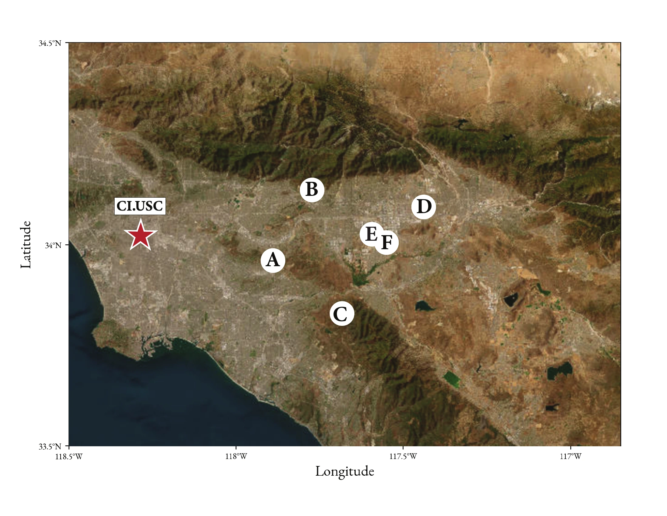
At CI.USC, several earthquakes east of Los Angeles produce a late transverse Love-wave packet that is weak or absent in both simulations. The event map links the waveform examples to their source locations. The highlighted intervals identify the arrivals behind the mismatch.
This is a specific target for model improvement: reproduce the observed surface-wave propagation into the basin, alongside the amplitude and duration constraints.
Detailed methods
Spectral-element simulation setup
The simulation domain spans 225 × 130 × 25 km, with a maximum modeled frequency of 1 Hz and a minimum shear-wave speed of 500 m/s. The meshes contain roughly 1.8 million elements. The study required about 2,700 GPU hours on USC’s high-performance computing cluster. Matching the setup between models makes their different velocity structures the central comparison.
Choose metrics that measure different waveform properties
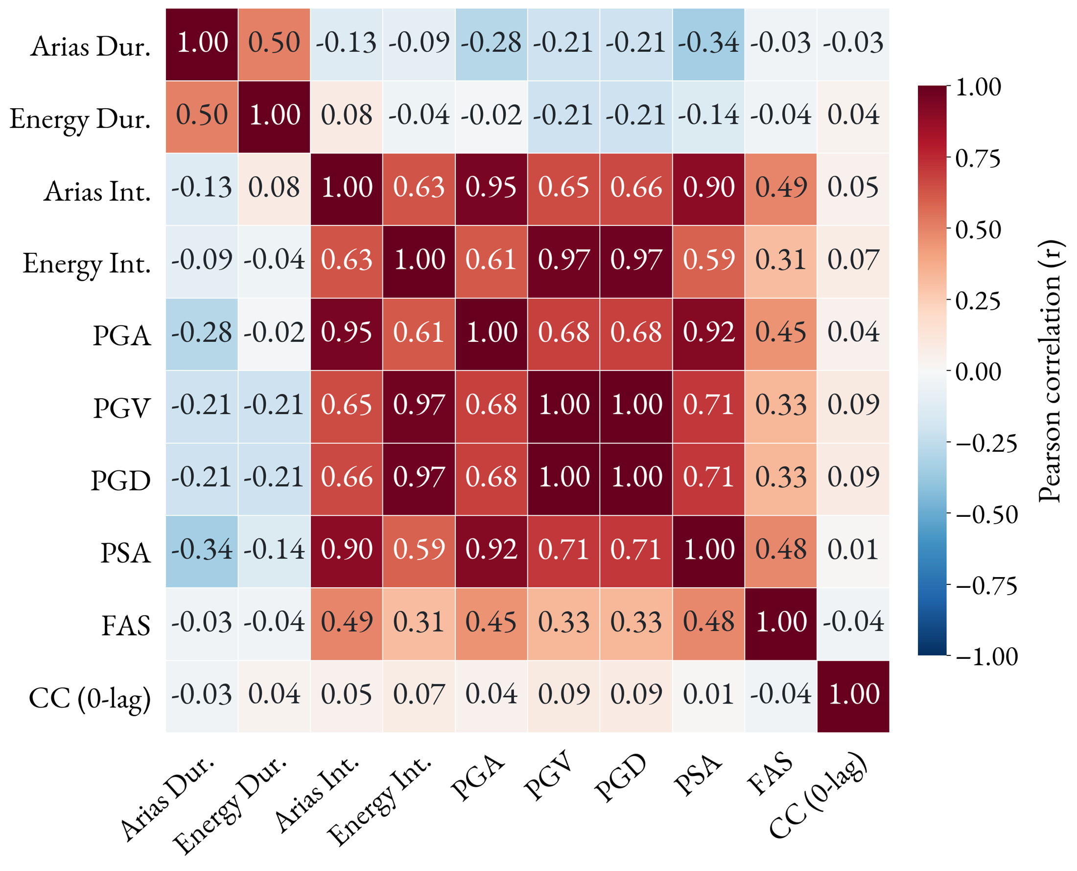
The first matrix shows why averaging many conventional goodness-of-fit metrics can overweight the same underlying amplitude information. I selected peak ground acceleration, Arias duration, Fourier amplitude spectra, travel-time delay, and delay-corrected cross correlation to span a broader set of waveform properties. Pseudo-spectral acceleration supplies an additional quantity relevant to engineering.
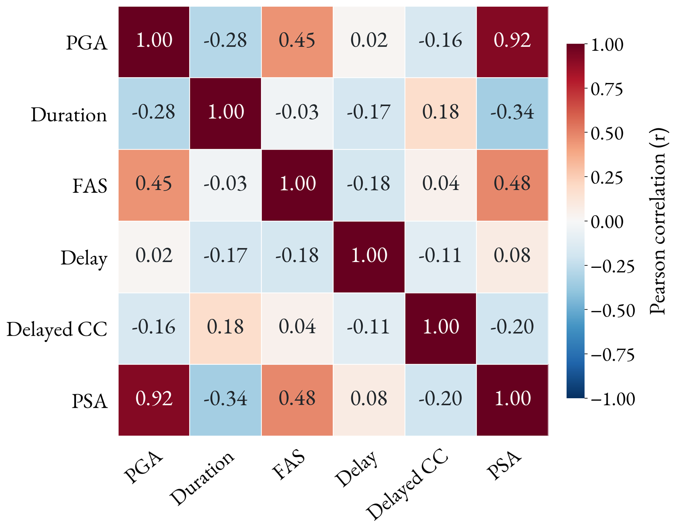
The second matrix shows the reduced overlap among the selected diagnostics, while also making the remaining strong PGA–PSA correlation explicit.
Construct basin-to-reference amplification factors
For each event, I selected comparable hard-rock stations outside the basin and measured horizontal peak ground acceleration. I corrected for distance differences, formed station-to-reference factors, and aggregated them over basin stations and events. The same comparison framework supports examination of source direction and spectral period. The reference-site approach draws on Boore et al. (2006), Wirth et al. (2019), and Jayaram and Baker (2008).
Why it matters
The study provides specific benchmarks for improving velocity models and evaluating their use in hazard assessment. A useful model update should improve the waveform feature and region it targets without hiding poorer performance elsewhere.