Dense-array seismology

Shallow Subsurface Imaging in the Nepal Himalaya

Applying my GDANT method to dense seismic observations to image shallow structure beneath the Melamchi Valley and investigate its links to mountain hydrology.

Seismic Imaging
Hydrology
Landslides

Research question

How does subsurface structure vary beneath a Himalayan ridge, and how do those variations relate to fracturing, weathering, and the scale of observation?

Study design

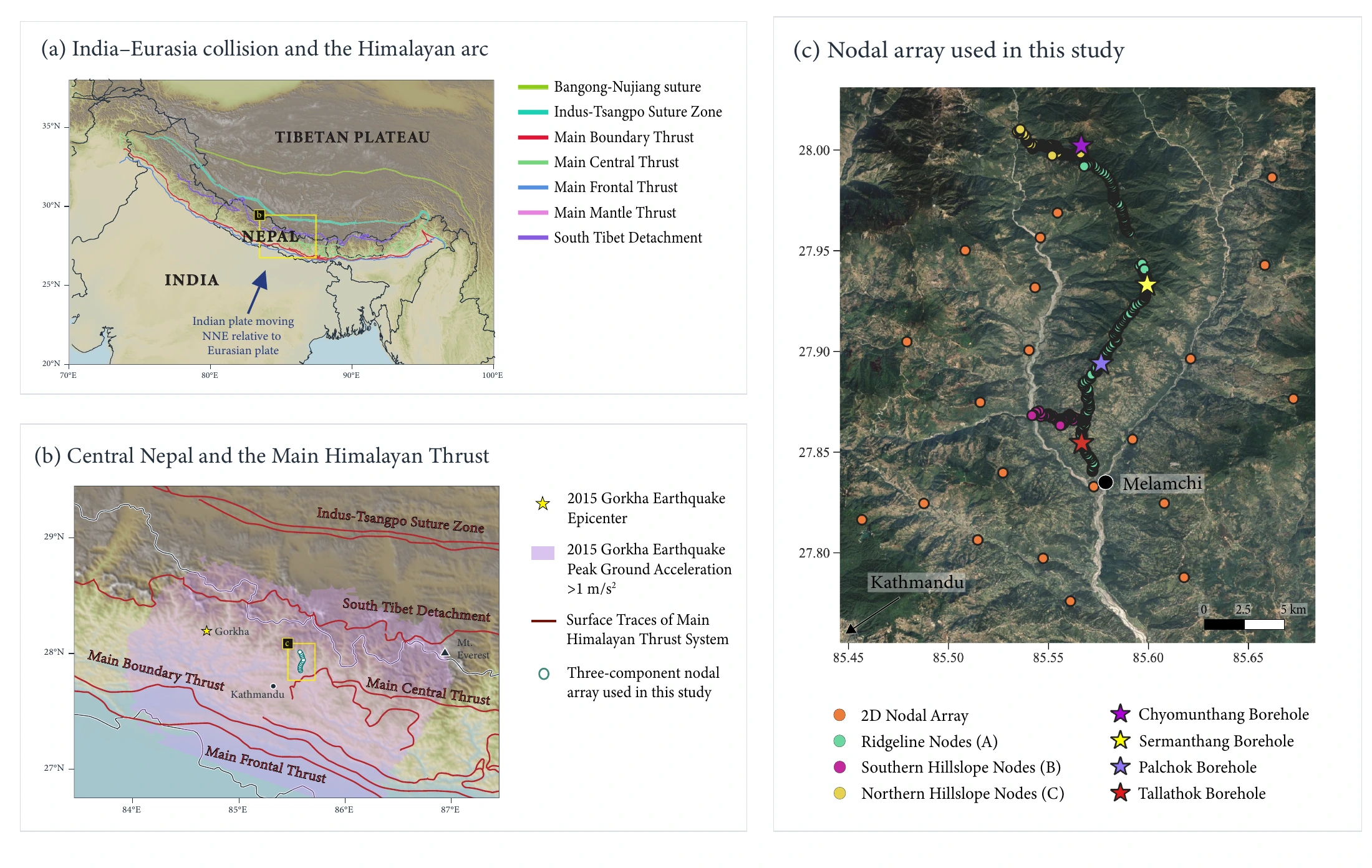
I designed and carried out the ridge-scale seismic imaging study using the GDANT method I developed. I used continuous records from 165 three-component geophones in the Melamchi Valley, together with topographic forward modeling, finite-frequency kernels, and iterative inversion, to recover a shallow shear-wave velocity profile.

Within the wider Nepal FRES collaboration, I compared this ridge-scale image with measurements of the upper tens of meters, borehole observations, and regional tectonic and exhumation evidence.

Three-panel map showing the Himalayan collision, central Nepal faults and Gorkha earthquake setting, and the Melamchi nodal array with ridgeline, hillslope, and borehole sites. — The maps connect the Himalayan tectonic setting to the local array. The ridgeline deployment and nearby hillslope and borehole observations make it possible to compare structure across spatial scales.

Key findings

The ridge interior is faster in the south and slower in the north
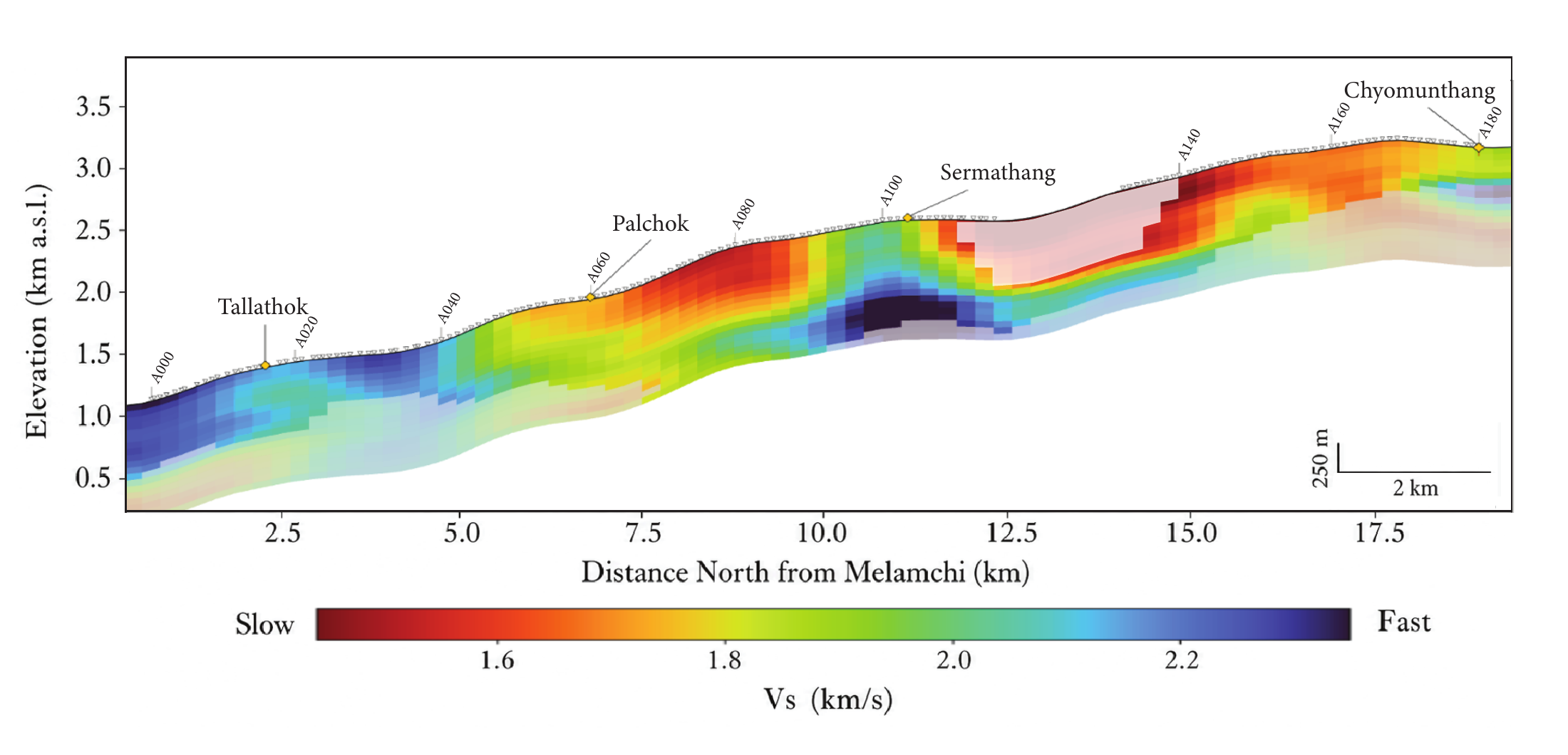
The profile resolves a northern low-velocity layer extending several hundred meters below the surface, alongside faster material at depth and a localized fast body beneath Sermathang.
The upper tens of meters show the opposite trend
Shallow surface-wave measurements generally show slower material toward the south and faster material toward the north. The two methods sample different depths and different rock volumes.
Exhumation and fracturing connect the two scales
I developed a physical explanation in which southern surface weathering and northern fracture damage produce contrasting velocity patterns at shallow and ridge-interior scales.

Image the ridge below the critical zone

The GDANT profile fills the gap between very shallow surveys and regional crustal models. It resolves the ridge interior while accounting for the steep surface topography.

The broad south-to-north contrast is accompanied by local structure: a faster body beneath Sermathang and faster material beneath the northern slow layer. Masked portions of the section identify regions poorly resolved by the array geometry.

Red and orange mark lower shear-wave speeds, while blue marks higher speeds. The color scale spans 1.4–2.4 km/s. Masked regions have low resolution because of the array geometry. These contrasts extend beneath the near-surface zone sampled by shallow surveys.

Compare measurements at different depth scales

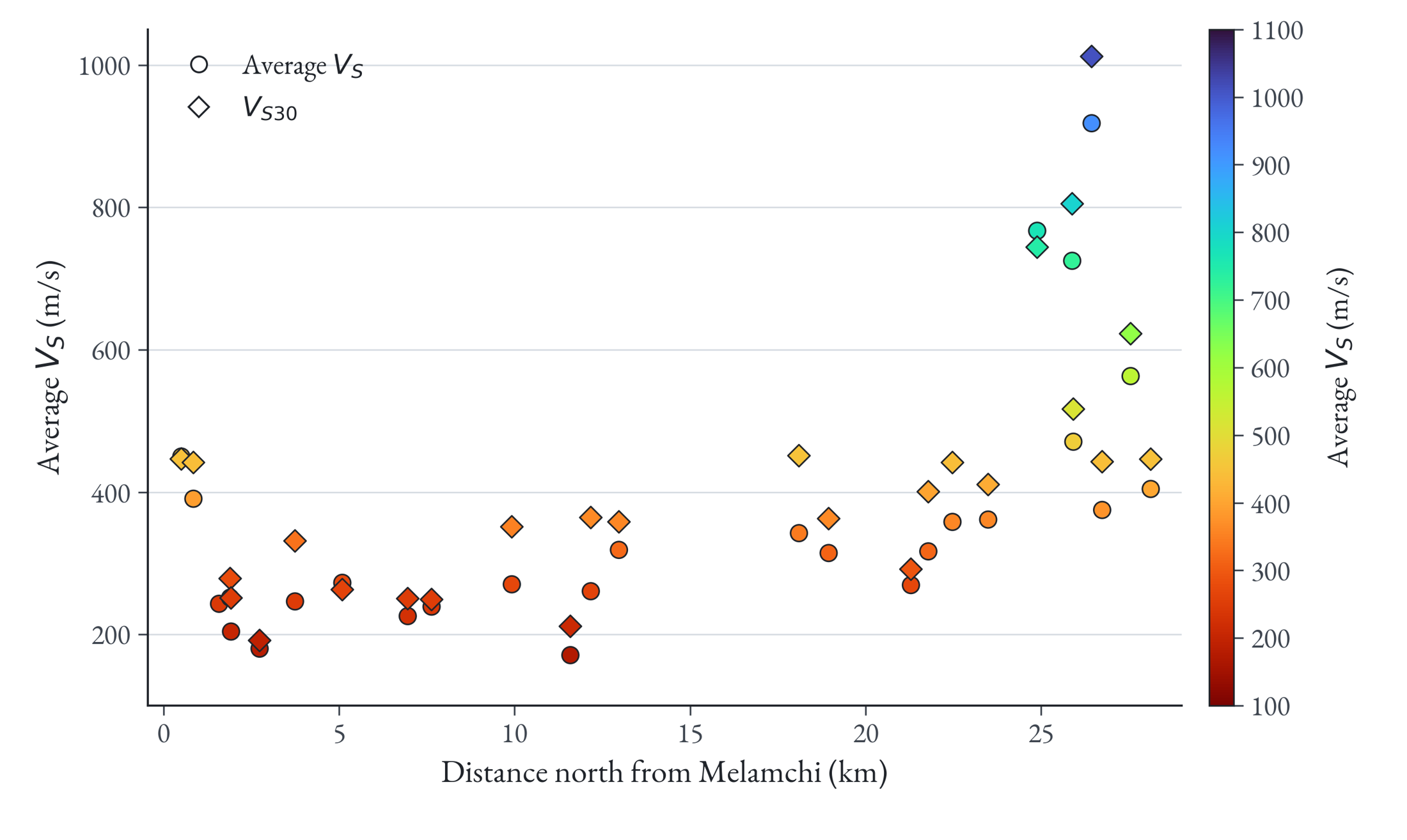
Multichannel analysis of surface waves (MASW) characterizes roughly the upper 15–30 m at individual sites. Those measurements generally show lower velocities in the south and higher velocities in the north. The ridge-scale image shows the opposite broad pattern.

The contrast is the central observation: near-surface material and the deeper ridge interior record different aspects of rock transformation.

Shallow average shear-wave velocity and Vs30 versus distance north from Melamchi, with higher values at many northern sites. — Site-scale MASW measurements provide the shallow comparison to the GDANT profile above. Data are from Medwedeff et al. (2022).

Link the velocity contrasts to rock transformation

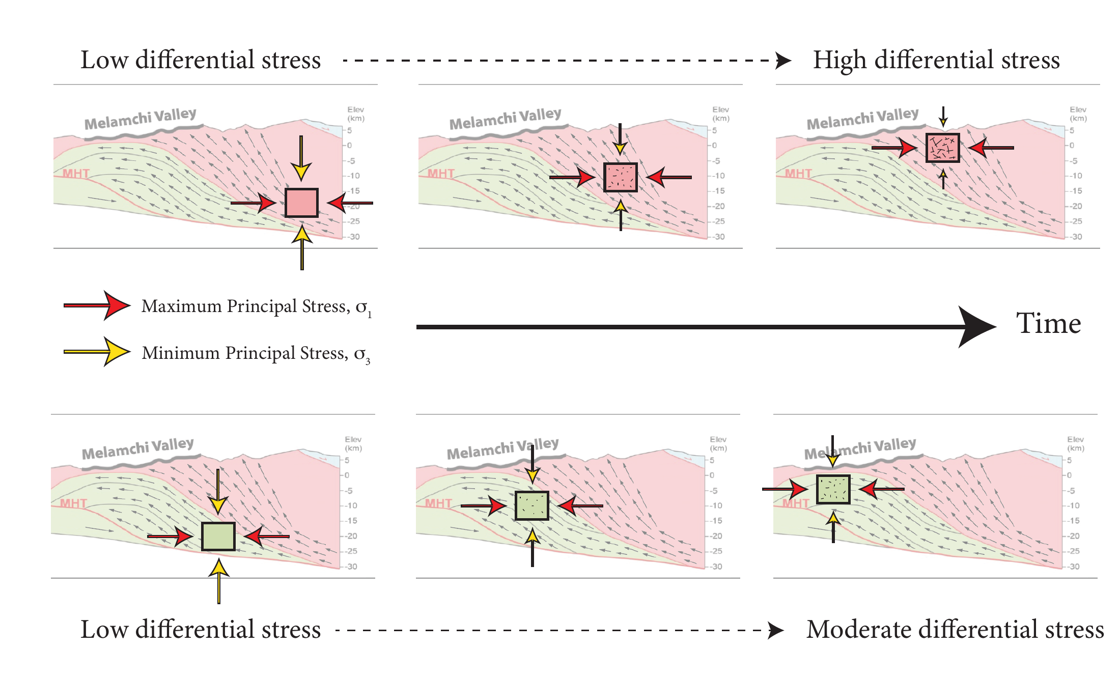
I relate these observations to a northward increase in uplift and exhumation. As rock moves toward the surface, unloading changes the balance between principal stresses. Greater differential stress can promote microcracking and the development of connected fracture networks.

The stress-history schematic illustrates this mechanism. The interpretation draws on Leith et al. (2014), with the regional section modified from Pandey (1995).

Two schematic exhumation histories showing changes in principal stresses as rock rises toward the surface, producing high versus moderate differential stress. — Different exhumation paths produce different stress histories. The proposed mechanism connects tectonic unloading with fracture development in the ridge interior.

A physical explanation for the opposite trends

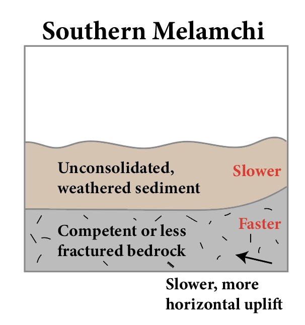
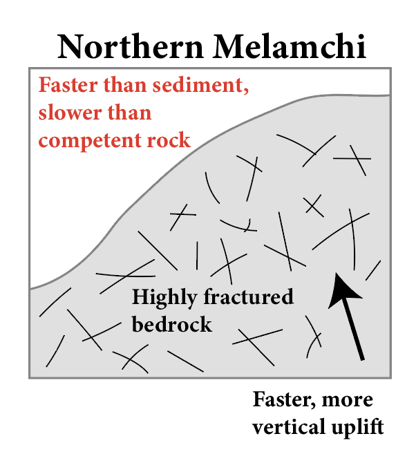
In the south, loose and weathered surface material can overlie a comparatively competent, faster ridge interior. In the north, exposed rock can be faster than southern soil at the surface while distributed fractures lower the velocity of the larger rock volume below.

These conceptual sections reconcile the observations at both scales and connect the seismic image to questions about water flow through fractured mountain bedrock.

Conceptual southern Melamchi section with slow unconsolidated weathered sediment over faster, less fractured bedrock. — Southern ridge: a slow surface layer overlies a comparatively fast interior.

Conceptual northern Melamchi section with highly fractured bedrock and stronger vertical uplift. — Northern ridge: exposed fractured rock is faster than loose sediment but slower than competent bedrock.

Detailed methods

The imaging workflow

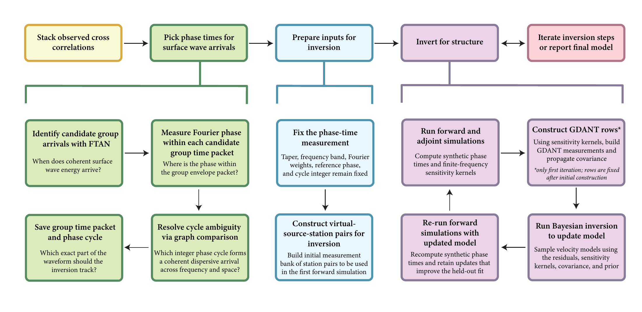
I begin with stacked ambient-noise cross correlations and identify candidate surface-wave packets. After selecting consistent phase measurements, I use forward and adjoint simulations to compute phase times and finite-frequency sensitivity kernels. GDANT rows and their covariance then enter the Bayesian model update.

The designed rows are fixed after their initial construction. Each updated model is evaluated with new forward simulations, retaining updates that improve the fit to held-out observations.

Workflow connecting stacked cross correlations, phase picking, fixed measurement definitions, forward and adjoint simulations, GDANT row construction, Bayesian inversion, and held-out validation. — The workflow separates phase selection, measurement design, and iterative model updates. GDANT rows are constructed in the first iteration and retained thereafter.

Identify coherent wave packets with Fourier phase

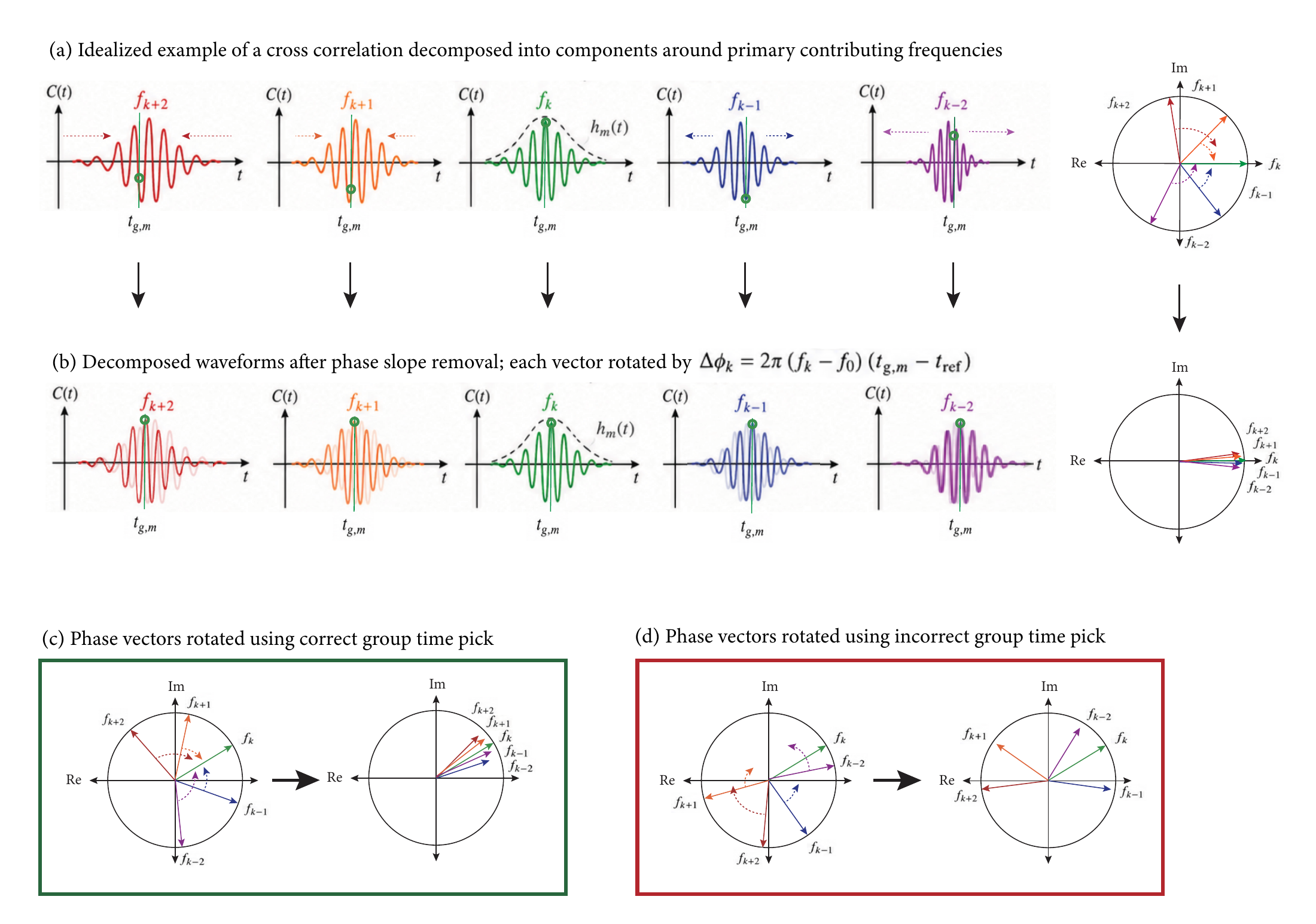
Frequency–time analysis identifies candidate group arrivals. Fourier phase then helps determine which packet contains coherent energy across neighboring frequencies and which phase cycle lies within that packet.

The schematic shows how removing the phase slope aligns the frequency components when the group-time choice is consistent. Once selected, the packet, phase cycle, taper, frequency band, and Fourier weights define the measurement tracked through the inversion.

Cross-correlation decomposed into frequency components, with phase-vector rotations comparing correct and incorrect group-time choices. — Consistent group timing aligns the phase vectors across frequency. This provides a way to evaluate candidate arrivals before inversion.

Resolve phase-cycle ambiguity across frequency and space

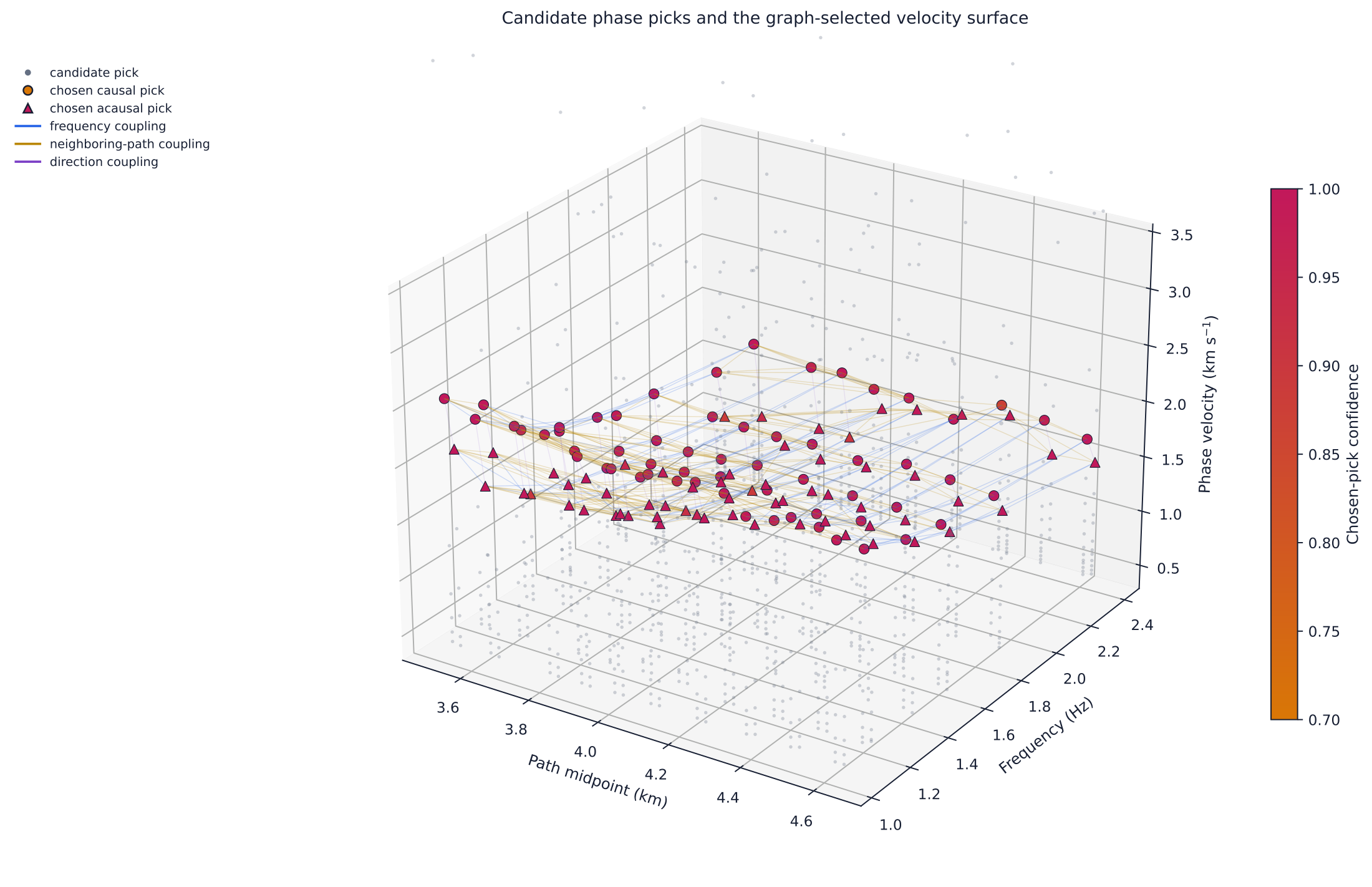
Individual phase-time candidates can differ by whole cycles. I compare candidates across neighboring frequencies and station-pair midpoints, including their propagation directions, to select a coherent dispersive arrival. The graph connects these related measurements so the chosen phase times remain consistent in frequency and space.

Candidate phase picks and a graph-selected phase-velocity surface plotted against frequency and path midpoint, with causal and acausal picks distinguished. — The selected picks form a coherent surface across the measurement bank, rather than a collection of unrelated single-frequency choices.

Evaluate spatial resolution

Point-spread tests characterize how a compact anomaly appears after inversion. The dissertation’s tests give lateral widths of approximately 1.1–1.3 km and vertical widths of 0.3–0.5 km. I use that scale to distinguish broad features of the ridge interior from thin layers and sharp boundaries that the imaging smooths.

Why it matters

The study connects near-surface measurements with structure at the scale of an entire ridge. That intermediate view helps investigate how rock condition, long-term tectonic forcing, and short-lived hydrological events interact in a steep mountain landscape.